


Skip to content

Free and open source

MIT license. Free to use, change and share. Source on GitHub.

Detecting manipulated faces in video.

xdfdet compares nine ways to train an EfficientNet-B4 face manipulation detector, measuring detection performance, probability reliability and the face regions associated with its predictions.

By senior AI researcher Mert Kaya and Venera Adanova, TED University · Presented at UBMK 2026 in Istanbul and published in IEEE Xplore.

CodeModelsThesis

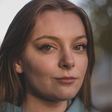
A heatmap (Grad-CAM) from the detector trained with altered images and black filled patches. On this real portrait, it highlights the eyes and eyebrows and predicts real.Photo: Pexels

How the study works

In high-stakes settings, a detector’s verdict helps only when someone can check it.

  1. 1

    Faces from 2,000 videos

    We use a widely used deepfake video dataset (FaceForensics++): 1,000 real videos, each paired with a manipulated copy. We detect, align and crop the faces.

    Real frame
    Manipulated frame
  2. 2

    Nine training setups

    We train the same detector (EfficientNet-B4) in nine setups, three runs each. We vary altered training images (data augmentation) and filled patches over parts of the face (cutout).

    Cutout on a fake frame
    Star cutout on a real frame
  3. 3

    Explaining each decision

    Heatmaps (Grad-CAM) show image regions associated with each prediction. We measure their intensity in eight face regions.

    Grad-CAM activation
    Eight face regions
Full pipelineFace preparation, prediction and explanation in seven steps

Each image is the output of the xdfdet code on a real Pexels portrait. The FaceForensics++ examples come from the thesis.

  1. 01

    Face detection

    A face detection tool (MTCNN) aligns and crops faces. The model uses 12 evenly spaced frames from each video.

    Detected face and eyes
    Aligned crop
  2. 02

    Facial landmarks

    A face analysis library (dlib) marks the points used to define eight face regions.

    68 landmarks and region outlines
    Region masks as scored. The jaw polygon closes across the lower face, so the jaw score overlaps the nose and mouth.
  3. 03

    Image similarity (SSIM)

    A similarity map compares each manipulated frame with its real source. Dark areas are nearly identical and guide patch placement.

    Real frame
    SSIM difference
    Manipulated frame

    FaceForensics++ frames, from the thesis

  4. 04

    Filled patches (cutout)

    On fake frames, a landmark polygon over the most similar area is filled with black, white or random pixels. Real frames get a star with a radius of 8 to 15 pixels and the same fill.

    Black fill
    White fill
    Random fill
    Star on a real frame
  5. 05

    Altered training images (augmentation)

    The Albumentations library adds noise, blur, color shifts, flips and small rotations. The intense setting applies them four to five times as often.

    Input
    Standard, one random draw
    Intense, one random draw
  6. 06

    Video-level prediction

    The face manipulation detector (EfficientNet-B4) scores 12 frames and averages them into one video score. Below 0.5 means fake.

    12 face crops
    EfficientNet-B4 per frame
    12 frame scores
    Mean
    0.9997
    Video score
  7. 07

    Grad-CAM

    This heatmap method highlights regions associated with a prediction. We average maps from three frames and measure them in each face region.

    Input
    Grad-CAM, augmentation and black fill

What we found

We measure separation of real and fake videos (AUC), classification at one threshold (F1), and probability errors (Brier score and log loss).

Altered images and black patches improve detection

The augmentation and black-fill cutout detector outperforms the baseline detector on all four measures.

Augmentation and black-fill cutout: AUC 0.8971. Baseline: 0.8678. Both are means of three runs; 1.0 means perfect separation and 0.5 means chance.

Metrics disagree

The standard-augmentation detector ranks last on AUC and second on F1. The measures assess different aspects of detection.

Augmentation with random-fill cutout has 0.4656 log loss. Augmentation with black-fill cutout has 0.8971 AUC.

In more detailCalibration

Calibration describes how closely probabilities match observed outcomes, for example whether predictions of 90% are correct about nine times in ten. Brier score and log loss measure probability errors.

Why detectors need itThis helps readers assess how much to trust a probability.

Dot: mean of three runs. Line: one standard deviation. ↑ higher is better, ↓ lower is better. FaceForensics++ test split of 150 video pairs.

Testing on a different video dataset

A check run after the paper, on 398 unseen videos from the Deepfake Detection Challenge (DFDC): the same eight models reach AUC 0.60 to 0.66, against 0.86 to 0.90 on FaceForensics++, and catch 15% to 36% of the fakes.

Kaggle notebook

A hidden trade-off in the nose region

The nose is among the most active regions in both right and wrong decisions.

The paper shows that aggregate detection scores can hide reliance on particular face regions.

One face, four setupsHeatmaps and face-region measurements on one portrait

All four call this portrait real, yet they look at different places. The augmentation and black-fill setup focuses on the eyes and eyebrows; black-fill cutout alone barely activates.

Baseline

Probability of being real 0.9947

Heatmap activation by region (Grad-CAM, 0 to 100)

  • Outer mouth47
  • Inner mouth47
  • Jaw44

Standard augmentation

Probability of being real 0.9999

Heatmap activation by region (Grad-CAM, 0 to 100)

  • Left eyebrow84
  • Left eye84
  • Right eye78

Cutout, black fill

Probability of being real 0.7315

Heatmap activation by region (Grad-CAM, 0 to 100)

  • Left eye7
  • Left eyebrow6
  • Jaw1

Augmentation + black fill

Probability of being real 0.9999

Heatmap activation by region (Grad-CAM, 0 to 100)

  • Left eye79
  • Left eyebrow74
  • Nose67

One portrait is an example. The paper averages Grad-CAM over the test videos in four groups: fakes caught, fakes missed, real videos accepted and real videos flagged as fake.

All nine setupsTraining image changes and filled patches, with detection scores (AUC)

Augmentation: None

No cutout

0.8678

Augmentation: Flips only

Random fill

0.8711

Black fill

0.8666

White fill

0.8639

Augmentation: Standard

No cutout

0.8610

Random fill

0.8837

Black fill

0.8971
highlighted setup

White fill

0.8734

Augmentation: Intense

No cutout

0.8718

AUC as reported in the paper. The cutout-only setups still used random horizontal flips, although the paper lists them without augmentation.

Test your own eye

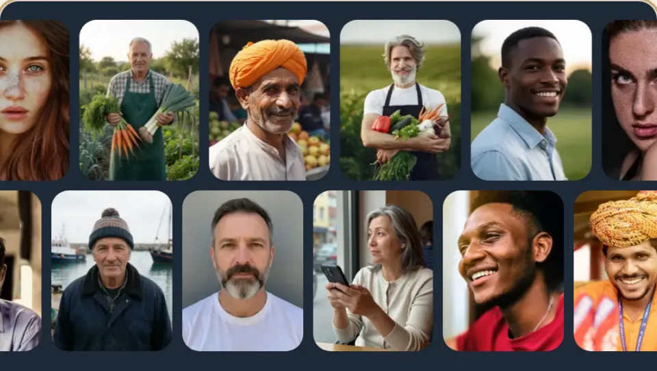
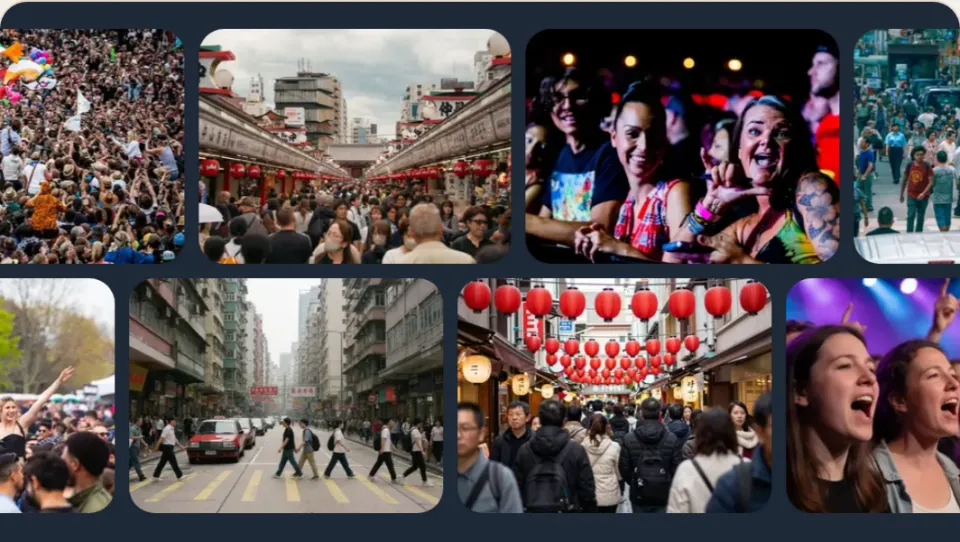
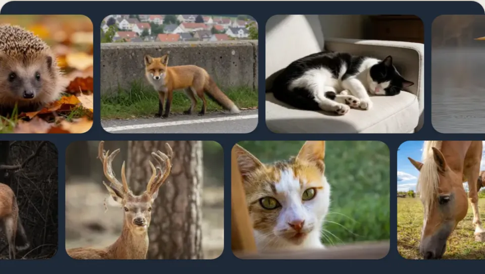
Distinguish real photos, screenshots and clips from AI-generated ones, then estimate figures about media made or altered by AI.

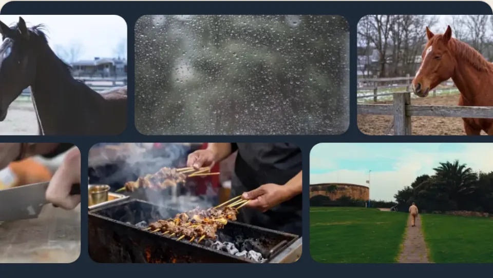
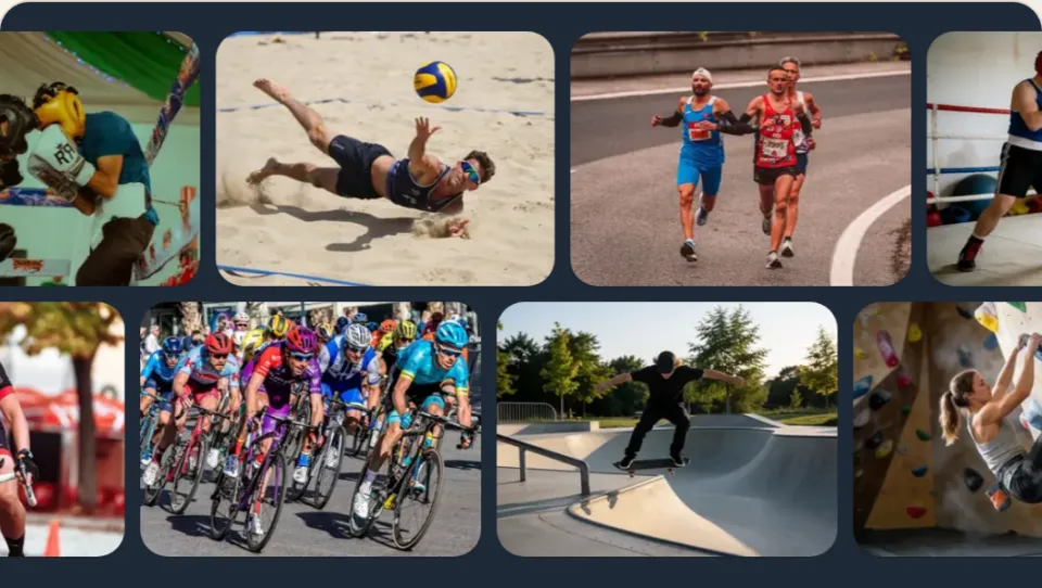
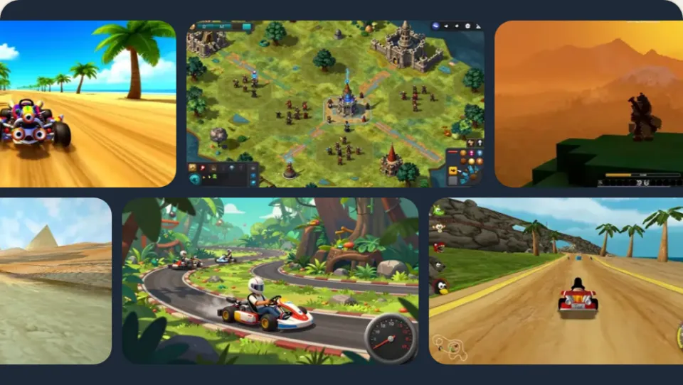
PortraitsCrowdsAnimalsLandscapesVideo clipsSportsAnimationVideo gamesWebsites

Score a video

Two commands, no dataset needed. The weights download from Hugging Face on first use.

  1. 1

    Install

    Python 3.11 to 3.13.

    pip install git+https://github.com/mertkayacs/xdfdet
  2. 2

    Run on a video

    Prints the probability of being real and the verdict, and saves a heatmap with face-region measurements.

    xdfdet predict video.mp4 --gradcam cam.png
Reproduce the studyNeeds the research dataset and a graphics processor (GPU)
  1. 3

    Get the data

    Request FaceForensics++ from its authors. It is licensed for research only.

  2. 4

    Crop the faces

    32 frames per video, 224×224 pixels.

    xdfdet crop raw/ faces/
  3. 5

    Train

    Pick one of the nine setups. A Colab T4 GPU is enough.

    xdfdet train --data faces/ --config aug-cutout-black --out model.keras
  4. 6

    Evaluate and explain

    The four metrics, plus Grad-CAM per region for right and wrong predictions.

    xdfdet evaluate --data faces/ --model model.keras
    xdfdet analyze --data faces/ --model model.keras --out regions.json

Before comparing numbers, read the notes on the original runs. Each original run drew its own random data split.

Trained modelsEight detectors, CC BY-NC 4.0, for non-commercial research.

The nine setups, in numbers

These scores compare the nine setups in this study. AUC measures ranking across thresholds; F1 measures classification at the chosen threshold.

AUC, augmentation plus black-fill cutout; mean over 3 runs
0.8971 ± 0.0064
Source
F1 for the same setup; mean over 3 runs
0.8429 ± 0.0101
Source
Released EfficientNet-B4 models, CC BY-NC 4.0
8
Source
FaceForensics++ videos: 1,000 real and 1,000 manipulated
2,000
Source
Unseen DFDC videos tested; model AUC ranges from 0.60 to 0.66
398
Source
Detection accuracy falls when these models are tested on unseen videos.

The original notebook runs used separate, unseeded test splits for each configuration. The paper's three-run averages differ from the released checkpoints' single-run scores. Grad-CAM shows regions associated with a prediction; a heatmap does not prove that a video is authentic.

Cite this studyMSc thesis DOI and the published IEEE UBMK 2026 paper
@inproceedings{kaya2026augmentation,
  title     = {Augmentation and Cutout in Deepfake Detection: A Comparative Study of
               Accuracy, Calibration, and Attention},
  author    = {Kaya, Mert and Adanova, Venera},
  booktitle = {2026 11th International Conference on Computer Science and Engineering (UBMK)},
  pages     = {78--83},
  year      = {2026},
  publisher = {IEEE},
  doi       = {10.1109/UBMK71847.2026.11745298},
  url       = {https://ieeexplore.ieee.org/document/11745298}
}

@mastersthesis{kaya2025xdfdet,
  title  = {Explainable Deepfake Detection Using Frame Level CNN Models:
            A Comparative Study of Augmentation and Cutout Techniques},
  author = {Kaya, Mert},
  school = {TED University},
  year   = {2025},
  doi    = {10.5281/zenodo.18998566}
}

Questions about explainable deepfake detection

How do the nine xdfdet training setups compare?

Augmentation plus black-fill cutout reaches 0.8971 mean AUC across three FaceForensics++ runs, compared with 0.8678 for the baseline EfficientNet-B4. That comparison covers this experiment. On 398 unseen DFDC videos, the released models reach only 0.60 to 0.66 AUC, so the evaluation dataset changes the result substantially.

How does xdfdet explain a deepfake prediction?

xdfdet uses Grad-CAM heatmaps to show image regions associated with each prediction. The analysis measures activation in eight facial regions defined by 68 landmarks, including the eyes, eyebrows, nose, mouth and jaw. Heatmaps help you inspect a detector's behavior. They do not establish the cause of a manipulation or guarantee that the verdict is correct.

Can I download the xdfdet models and run them locally?

Eight EfficientNet-B4 models are available on Hugging Face and Kaggle. Install the Python package from the GitHub repository and run xdfdet predict on a video to obtain a real probability, a verdict and an optional Grad-CAM image. The package supports Python 3.11 to 3.13. Model weights download on first use; inference does not require the training dataset.

Is xdfdet free for commercial deepfake detection?

The xdfdet code uses the MIT license, while the eight released model checkpoints use CC BY-NC 4.0. The weights were trained on FaceForensics++, whose terms restrict use to non-commercial research. You can inspect the code and study the models for research. Commercial use of the released weights requires permission from the relevant rights holders.

Which dataset and model architecture does xdfdet use?

The study uses 2,000 FaceForensics++ videos: 1,000 real videos paired with 1,000 manipulated copies. MTCNN finds and aligns faces before cropping them to 224 by 224 pixels. EfficientNet-B4 scores 12 frames independently and averages their scores for the video prediction. Nine training setups change augmentation and cutout while keeping the underlying architecture fixed.

Where can I cite the xdfdet thesis and UBMK paper?

Mert Kaya's 2025 MSc thesis at TED University has DOI 10.5281/zenodo.18998566. The paper by Mert Kaya and Venera Adanova, Augmentation and Cutout in Deepfake Detection: A Comparative Study of Accuracy, Calibration, and Attention, was presented at UBMK 2026 in Istanbul and published in IEEE Xplore on pages 78 to 83. Its DOI is 10.1109/UBMK71847.2026.11745298. Use the BibTeX entries on this page.